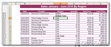
 The Subtotals command in Excel offers a very quick of getting, well, subtotals – sums, averages and more- without the use of functions and formulas.
If you can read these instructions or watch the video, you will know how to calculate subtotals for the hugest, most humongous lists. But you must sort the table or database first. I said, you must sort the table. That’s right, don’t forget to sort first.
Video: Super easy subtotals in a Microsoft Excel database
Step 1 – Sort the database
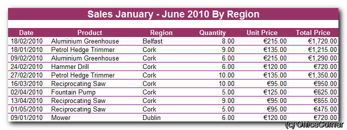
Make sure you have a database first and then if you want to have a total by Region, sort by Region.
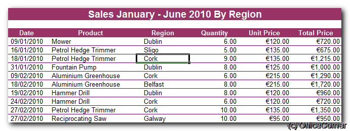
As long as you have no blank rows or blank columns in your list or table, just click inside the column to sort by and then click the Sort command.
Step 2 – Subtotals
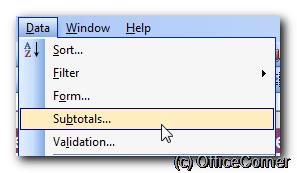
Click any cell within your database and select Subtotals from the Data menu
Now read carefully the instructions in the dialog box.
- Under At each change in make sure that you select the same field name (column heading) as in Step 1.
- For Use function choose from the dropdown. Usually, Sum is used but you can easily get an average or other calculation of your choice.
- Add subtotal to lets you choose which column(s) you want to add up or average so choose as few or as many as you need.
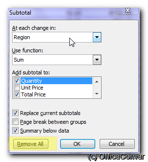
Click OK to see the result. Notice the outlining on the left hand side. 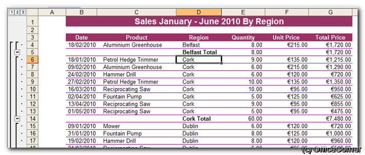
Step 3 – Outlining
 Click the symbols (-, + and the figures 1, 2, 3 to the left hand side of the spreadsheet) to display or hide various levels of details in the database.

Step 4 – Remove All Subtotals
To remove the subtotals, select Subtotals in the Data menu. Click Remove All in the dialog box.


